Introduction
Tax increment financing (TIF) is a tool used to promote economic development in specific areas. It allows a municipality to re-invest all new property tax revenue back into the area from which it came. TIF districts last for 23 years, with the option to extend to 35 years.
TIFs work by “freezing” the value of all property within them at the time they are established. Any “new” property value created within the TIF (whether through development or rising prices) is taxed as usual. However, the tax revenue generated by any new value over the frozen amount is diverted into the TIF fund, which is then allocated for specific projects.
TIFs do not increase tax bills directly; they do not change levies or tax rates. However, TIFs can indirectly affect tax bills by capturing property value that would otherwise increase the tax base and, therefore, reduce rates. This effect is difficult to parse, since it requires recalculating bills using a counterfactual tax base.
Enter PTAXSIM. With some careful data manipulation, PTAXSIM can measure the impact of a TIF by recalculating bills as if the TIF hypothetically does not exist. This vignette demonstrates that process.
The Wheeling Town Center II TIF
Using PTAXSIM, we’re going to examine the impact of a single TIF: the Wheeling Town Center II (WTC2) TIF in Wheeling, IL. This TIF was established in 2014 and covers about 200 properties in downtown Wheeling. Since being established, its total increment (property value) has grown substantially, and it now receives about $5.5 million per year in tax revenue (as of 2020). We can determine the impact of the WTC2 TIF by recalculating historical tax bills as if it was never created.
First, load some useful libraries and instantiate a PTAXSIM database
connection with the default name (ptaxsim_db_conn) expected
by PTAXSIM functions.
library(DBI)
library(data.table)
library(dplyr)
library(ggplot2)
library(ggspatial)
library(glue)
library(here)
library(ptaxsim)
library(sf)

ptaxsim_db_conn <- DBI::dbConnect(RSQLite::SQLite(), here("./ptaxsim.db"))
Gathering PINs of interest
To determine the TIF’s impact, we first need a way to gather all the properties (PINs) in Wheeling. Fortunately, PTAXSIM’s database has all the data required to accomplish this task.
First, we’ll need to determine the Village of Wheeling’s agency
number. This is the ID used by the Clerk to track different taxing
bodies. To find Wheeling’s ID, we can directly query PTAXSIM’s database
and look in the agency_info table:
wh_agency_nums <- DBI::dbGetQuery(
  ptaxsim_db_conn,
  "SELECT agency_num, agency_name, minor_type
  FROM agency_info
  WHERE agency_name LIKE '%WHEELING%'"
)

wh_agency_nums
#>    agency_num                                        agency_name minor_type
#> 1   020290000                                      TOWN WHEELING   TOWNSHIP
#> 2   020290002                        GENERAL ASSISTANCE WHEELING   GEN ASST
#> 3   020290003                           ROAD AND BRIDGE WHEELING      INFRA
#> 4   031310000                                VILLAGE OF WHEELING       MUNI
#> 5   031310500         TIF - WHEELING - MILWAUKEE AVENUE CORRIDOR        TIF
#> 6   031310501    TIF - WHEELING - MILWAUKEE / MANCHESTER (SOUTH)        TIF
#> 7   031310502     TIF - WHEELING - MILWAUKEE / LAKE-COOK (NORTH)        TIF
#> 8   031310503                       TIF - WHEELING - TOWN CENTER        TIF
#> 9   031310504                         TIF - WHEELING - SOUTHEAST        TIF
#> 10  031310505                      TIF - WHEELING - SOUTHEAST II        TIF
#> 11  031310506                    TIF - WHEELING - TOWN CENTER II        TIF
#> 12  040040000 SCHOOL DISTRICT 21 WHEELING COMMUNITY CONSOLIDATED ELEMENTARY
#> 13  051080000                             WHEELING PARK DISTRICT       PARK
Here we can see the various taxing bodies around Wheeling and their
types. The agency number we want is 031310000 for the
VILLAGE OF WHEELING. With the agency number, we can find
all of the tax codes that make up
the municipality. To do so, we can again query PTAXSIM directly, this
time looking in the tax_code table:
wh_tax_codes <- DBI::dbGetQuery(
  ptaxsim_db_conn, "
  SELECT tax_code_num
  FROM tax_code
  WHERE agency_num = '031310000'
  AND year = 2020
  "
)
Finally, we can find all of Wheeling’s PINs with one last direct
query. This time we’ll look in the pin table using the tax
codes that make up Wheeling. We’ll use the glue library for
string expansion to make things a bit easier:
wh_pins <- DBI::dbGetQuery(
  ptaxsim_db_conn,
  glue_sql("
    SELECT pin, class
    FROM pin
    WHERE tax_code_num IN ({wh_tax_codes$tax_code_num*})
    AND year = 2020
    ",
    .con = ptaxsim_db_conn
  )
)
Mapping the area
Now that we have Wheeling’s PINs, we can use them to get a quick look
at the area using a map. First, we’ll get the PIN boundaries. These are
included in PTAXSIM’s database and can be retrieved using
lookup_pin10_geometry().
# PIN geometries only exist for 10-digit PINs, so we'll need to truncate our
# existing Wheeling PINs
wh_pin10s <- unique(substr(wh_pins$pin, 1, 10))

# The geometry is stored in the database as simple text, so we need to convert
# it to the correct type using sf
wh_pins_geo <- lookup_pin10_geometry(year = 2020, pin10 = wh_pin10s)
wh_pins_geo <- wh_pins_geo %>%
  st_as_sf(wkt = "geometry", crs = 4326)

# We'll also attach the first class code from each PIN14 to each PIN10 geometry
# and group them into broad buckets. This is just to help our visualization
wh_pins_geo <- wh_pins_geo %>%
  left_join(
    wh_pins %>%
      mutate(pin10 = substr(pin, 1, 10)) %>%
      group_by(pin10) %>%
      summarize(class = first(class)),
    by = "pin10"
  ) %>%
  mutate(
    major_class = substr(class, 1, 1),
    major_class_fct = recode_factor(
      major_class,
      "2" = "2 - Residential",
      "3" = "3 & 5 - Commercial",
      "5" = "3 & 5 - Commercial",
      "0" = "Other", "1" = "Other", "6" = "Other", "7" = "Other"
    )
  )
Next, we can get the municipality boundary for Wheeling from Cook Central, the County GIS data portal. Cook Central also has the boundaries for TIFs, so we can fetch the Wheeling Town Center II TIF boundary as well.
bound_muni <- st_read(paste0(
  "https://opendata.arcgis.com/api/v3/datasets/",
  "534226c6b1034985aca1e14a2eb234af_2/downloads/",
  "data?format=geojson&spatialRefId=4326&where=1%3D1"
), quiet = TRUE) %>%
  filter(MUNICIPALITY == "Wheeling")

bound_tif <- st_read(paste0(
  "https://opendata.arcgis.com/api/v3/datasets/",
  "8aeb00520c544aafb9a22510465c679d_18/downloads/",
  "data?format=geojson&spatialRefId=4326&where=1%3D1"
), quiet = TRUE) %>%
  # Pulled from the table of agency numbers above
  filter(AGENCY == 031310506)
Finally, we can plot the PINs, municipality boundary, and TIF boundary on a map.
Click here to show plot code
wh_pins_map <- ggplot() +
  annotation_map_tile(type = "cartolight", zoomin = -1) +
  geom_sf(
    data = wh_pins_geo,
    aes(fill = major_class_fct),
    alpha = 0.5,
    linewidth = 0.1
  ) +
  geom_sf(data = bound_muni, fill = "transparent", linewidth = 1) +
  geom_sf(
    data = bound_tif,
    fill = "purple2",
    color = "purple4",
    alpha = 0.3,
    linewidth = 0.9
  ) +
  annotation_scale(location = "br") +
  scale_fill_brewer(name = "", palette = "Set1") +
  guides(color = guide_legend(override.aes = list(size = 5))) +
  theme_void() +
  theme(
    legend.title = element_text(size = 14),
    legend.text = element_text(size = 12),
    legend.key.size = unit(24, "points"),
    legend.position = "bottom"
  )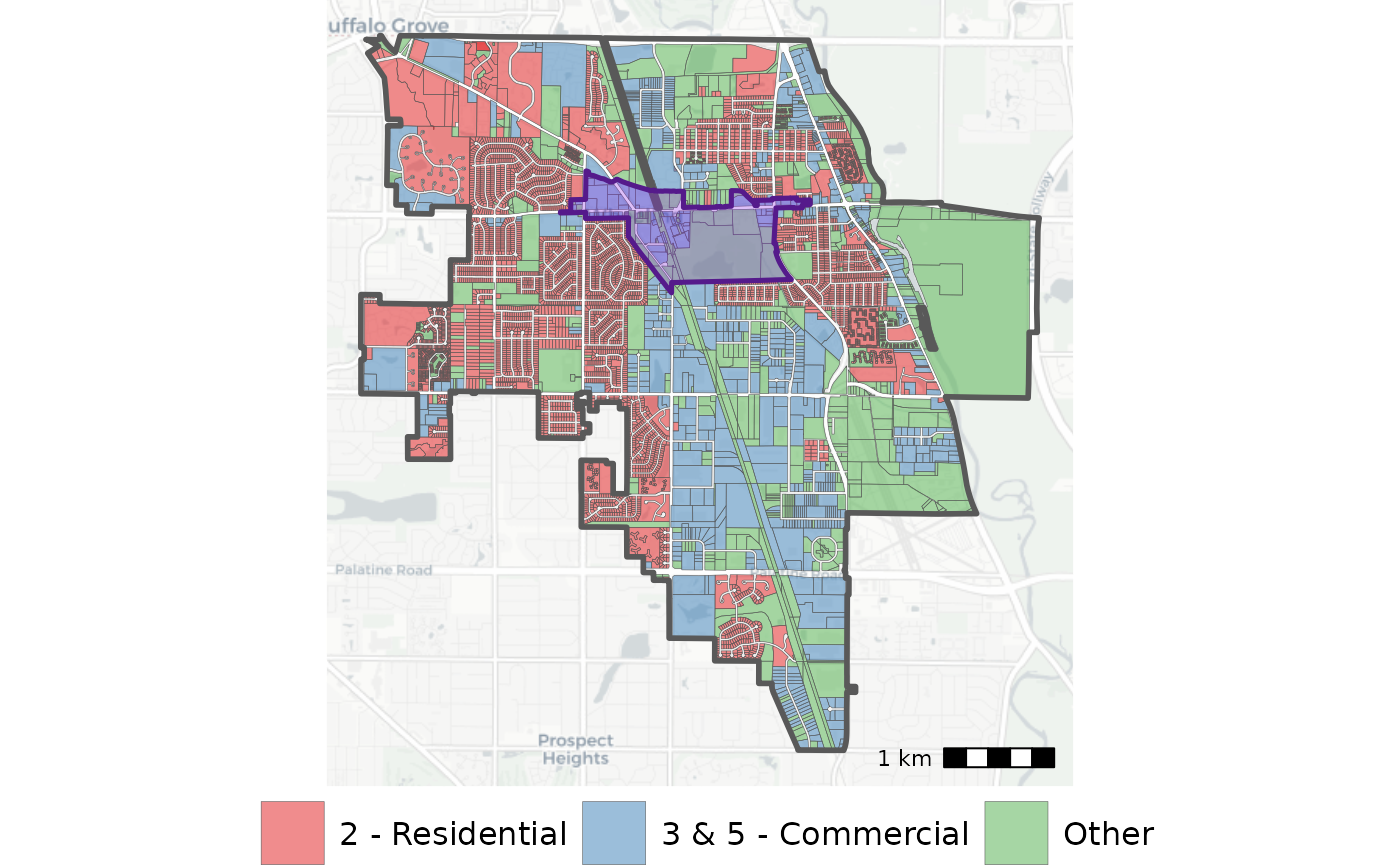
The map shows the TIF district highlighted in purple. It covers mostly commercial buildings and a small park. The primary development is called the Wheeling Town Center.
A quick aside: tax codes
The Wheeling Town Center II TIF was created by layering an additional taxing district boundary onto existing districts. When this happened, a new tax code was created. A tax code is a 5-digit number that identifies the unique combination of overlapping tax districts for a given area.
In 2014, the tax code for each PIN within the WTC2 TIF changed to represent their new, unique tax situation. This process is important to understand when dealing with TIFs, especially when calculating counterfactual scenarios.
Determining the increment
Now that we’ve mapped our TIF, it’s time to see how much taxable value (increment) it contains. We can do this by first gathering all PINs within the TIF, then comparing their total equalized assessed value to the value “frozen” by the TIF. Any property taxes on the value over the frozen amount go directly into the TIF fund.
We can use the TIF’s tax codes to find all the PINs within it. TIFs can have multiple tax codes, but the Wheeling Town Center II TIF only has one. We can use the agency ID for the TIF to look up its tax codes from the PTAXSIM database.
# TIF distributions will include all the unique tax codes that make up
# a TIF
tif_dists <- DBI::dbGetQuery(
  ptaxsim_db_conn, "
  SELECT *
  FROM tif_distribution
  WHERE agency_num = '031310506'
  "
)
Next, we can use the unique tax codes of the TIF to look up all of
its PINs. Then we can get the history of those PINs using PTAXSIM’s
lookup_pin() function.
tif_pins_vec <- DBI::dbGetQuery(
  ptaxsim_db_conn,
  glue::glue_sql("
    SELECT DISTINCT pin
    FROM pin
    WHERE tax_code_num IN ({unique(tif_dists$tax_code_num)*})
  ",
    .con = ptaxsim_db_conn
  )
) %>%
  pull(pin)

tif_pins_dt <- lookup_pin(2006:2020, pin = tif_pins_vec) %>%
  mutate(tax_code = lookup_tax_code(year, pin))
We can determine the amount of increment by comparing the total property value in the TIF (in EAV) to the frozen amount. Anything above the frozen amount is taxed by the TIF.
tif_pins_summ <- tif_pins_dt %>%
  group_by(year) %>%
  summarize(total_eav = sum(eav)) %>%
  left_join(tif_dists, by = "year") %>%
  mutate(amt_to_tif = total_eav - tax_code_frozen_eav)
Finally, we can plot the total EAV of all PINs in the TIF over time, highlighting the TIF start date and increment captured.
Click here to show plot code
# Create polygon to highlight the increment taxed by the TIF
plot_pin_fill <- tibble(
  x = c(2014, 2015, 2016, 2017, 2018, 2019, 2020, 2020),
  y = c(
    tif_pins_summ$total_eav[tif_pins_summ$year >= 2014],
    tif_pins_summ$total_eav[tif_pins_summ$year == 2014]
  )
)

tif_inc_plot <- ggplot(tif_pins_summ) +
  geom_area(
    aes(x = year, y = total_eav),
    fill = "grey50",
    alpha = 0.5
  ) +
  geom_polygon(
    data = plot_pin_fill,
    aes(x = x, y = y),
    fill = "purple2",
    alpha = 0.5
  ) +
  geom_vline(xintercept = 2014, linetype = "dashed", alpha = 0.7) +
  annotate(
    "text",
    x = 2013.7,
    y = 7.5e7,
    label = "Wheeling Town Center II\nTIF created",
    hjust = 1,
    size = 3.5,
    alpha = 0.5
  ) +
  annotate(
    "text",
    x = 2017.9,
    y = 5.5e7,
    label = "Increment to TIF",
    hjust = 1,
    size = 5,
    color = "purple2",
    alpha = 0.5,
    fontface = "bold"
  ) +
  scale_y_continuous(
    labels = scales::label_dollar(scale = 1e-6, suffix = "M"),
    expand = c(0, 0)
  ) +
  scale_x_continuous(n.breaks = 9, expand = c(0, 0.4)) +
  labs(x = "Year", y = "Total EAV of PINs in WTC2") +
  theme_minimal() +
  theme(
    axis.title = element_text(size = 13),
    axis.title.x = element_text(margin = margin(t = 6)),
    axis.title.y = element_text(margin = margin(r = 6)),
    axis.text = element_text(size = 11),
    axis.ticks.x = element_line(color = "grey70"),
    strip.text = element_text(size = 16),
    strip.background = element_rect(fill = "#c9c9c9"),
    legend.title = element_text(size = 14),
    legend.key.size = unit(24, "points"),
    legend.text = element_text(size = 12),
    legend.position = "bottom"
  )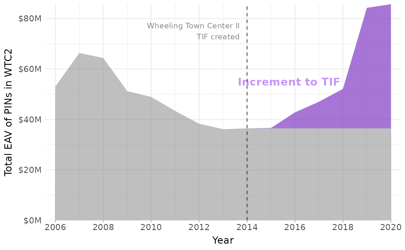
The plot shows the increment taxed by the TIF highlighted in purple. The flat grey area after 2014 represents the “frozen” EAV. Since 2014, the WTC2 TIF has doubled its total increment (purple + grey), with more than half of the new increment (purple) taxed by the TIF.
Tax revenue by district
Let’s look at how the change in increment has impacted the proportion
of each tax bill dedicated to the TIF. To do so, we can grab the tax
bill history of all PINs in the TIF using PTAXSIM’s
tax_bill() function.
tif_bills <- tax_bill(2006:2020, tif_pins_vec)Then do a quick aggregation to get the proportion of tax revenue dedicated to each district type. We’ll collapse some of the district types together to make plotting easier.
tif_bills_summ <- tif_bills %>%
  mutate(
    agency_minor_type = recode(
      agency_minor_type,
      "GEN ASST" = "MUNI",
      "PARK" = "MUNI",
      "INFRA" = "MUNI",
      "LIBRARY" = "MUNI",
      "MOSQUITO" = "MISC",
      "WATER" = "MISC"
    ),
    agency_minor_type = factor(
      agency_minor_type,
      levels = c(
        "TIF", "COOK", "MUNI", "TOWNSHIP", "MISC",
        "COMM COLL", "ELEMENTARY", "SECONDARY"
      )
    )
  ) %>%
  group_by(year, agency_minor_type) %>%
  summarize(total_rev = sum(final_tax))
Finally, we can plot the total tax revenue collected from the WTC2 TIF PINs, breaking out the total by district type.
Click here to show plot code
tif_dist_plot <- ggplot(data = tif_bills_summ) +
  geom_area(
    aes(x = year, y = total_rev, fill = agency_minor_type),
    alpha = 0.8
  ) +
  geom_vline(xintercept = 2014, linetype = "dashed", alpha = 0.7) +
  annotate(
    "text",
    x = 2013.7,
    y = 8e6,
    label = "Wheeling Town Center II\nTIF created",
    hjust = 1,
    size = 3.5,
    alpha = 0.5
  ) +
  scale_y_continuous(
    labels = scales::label_dollar(scale = 1e-6, suffix = "M"),
    expand = c(0, 0)
  ) +
  scale_x_continuous(n.breaks = 9, expand = c(0, 0.4)) +
  scale_fill_manual(
    name = "",
    values = c("#7d26cd", RColorBrewer::brewer.pal(7, "Set2"))
  ) +
  labs(x = "Year", y = "Total Tax Revenue from WTC2 PINs") +
  theme_minimal() +
  theme(
    axis.title = element_text(size = 13),
    axis.title.x = element_text(margin = margin(t = 6)),
    axis.title.y = element_text(margin = margin(r = 6)),
    axis.text = element_text(size = 11),
    axis.ticks.x = element_line(color = "grey70"),
    strip.text = element_text(size = 16),
    strip.background = element_rect(fill = "#c9c9c9"),
    legend.title = element_text(size = 14),
    legend.key.size = unit(24, "points"),
    legend.text = element_text(size = 12)
  )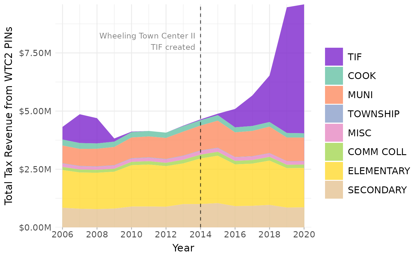
As of 2020, the WTC2 TIF captures about 55% of the total tax revenue collected from within its boundaries. This number will likely increase as the total EAV within the TIF continues to grow.
The plot also shows an earlier bump of revenue collected for a TIF district. This was the first Wheeling Town Center TIF, which was canceled in 2013.
Counterfactual scenario
Using PTAXSIM, we can also explore counterfactuals related to the WTC2 TIF that would otherwise be impossible to calculate. As an example, we’ll use PTAXSIM to determine the WTC2 TIF’s effect on the median tax bill in Wheeling by recalculating bills as if the TIF does not exist.
To do so, we must perform three steps:
- Update TIF distribution amounts
- Recalculate tax bases with EAV recovered from the TIF
- Recalculate bills with the the updated TIF distributions and tax bases
We can then plot the difference between real bills and the counterfactual bills to see the effect of the TIF over time.
1. Update TIF distribution amounts
First, we need to update the output of lookup_tif().
This function is an input to tax_bill() and contains a
column called tif_share, which indicates the percentage of
each bill dedicated to the TIF. To remove the share of the bill
dedicated to a TIF, we simply make this percentage equal to zero.
tif_dt_cntr <- lookup_tif(
  2006:2020,
  lookup_tax_code(2006:2020, wh_pins$pin)
) %>%
  # Set only the WTC2 TIF share to 0, leave all others untouched
  mutate(tif_share = ifelse(agency_num == "031310506", 0, tif_share))
2. Recalculate tax bases
Second, we need to alter the lookup_agency() output to
include EAV recovered from the removed TIF. This function is an input to
tax_bill() and contains the levy and base of each taxing
district in our area of interest. To remove the TIF, we need to first
calculate the difference between the total frozen EAV and the total
current EAV for each tax code in the TIF. We then take that difference,
sum it to the district level, and add the sum to each district.
# Get the unaltered levy and base for all PINs in Wheeling
tif_agency_cntr <- lookup_agency(
  2006:2020,
  lookup_tax_code(2006:2020, wh_pins$pin)
)

# For each agency and year, get the amount recovered from the TIF using the
# summary table we created earlier (tif_pins_summ)
tif_agency_amt_to_add <- tif_agency_cntr %>%
  filter(tax_code == "38228") %>%
  distinct(year, agency_num) %>%
  left_join(
    tif_pins_summ %>% select(year, amt_to_tif),
    by = "year"
  )

# Update the base by adding the recovered amount to the each district's tax base
tif_agency_cntr_updated <- tif_agency_cntr %>%
  left_join(tif_agency_amt_to_add, by = c("year", "agency_num")) %>%
  rowwise() %>%
  mutate(agency_total_eav = sum(agency_total_eav, amt_to_tif, na.rm = TRUE)) %>%
  select(-amt_to_tif) %>%
  setDT(key = c("year", "tax_code", "agency_num"))
3. Recalculate bills
Third, we can calculate counterfactual tax bills using our altered
inputs. All we need to do is pass the updated TIF share and district
base inputs to the tax_bill() function. We also create a
set of unaltered bills for comparison.
# Calculate unaltered, original bills for comparison
wh_bills <- tax_bill(2006:2020, wh_pins$pin)

# Calculate counterfactual tax bills where the WTC2 TIF does not exist
tif_bills_cntr <- tax_bill(
  year_vec = 2006:2020,
  pin_vec = wh_pins$pin,
  agency_dt = tif_agency_cntr_updated,
  tif_dt = tif_dt_cntr
)
Finally, we can plot the difference between median real bill and the median counterfactual bill to isolate the cost of the WTC2 TIF.
Click here to show plot code
tif_bills_cntr_summ <- wh_bills %>%
  group_by(year, pin) %>%
  summarize(`With TIF` = sum(final_tax)) %>%
  left_join(
    tif_bills_cntr %>%
      group_by(year, pin) %>%
      summarize(`No TIF` = sum(final_tax)),
    by = c("year", "pin")
  ) %>%
  tidyr::pivot_longer(ends_with("TIF")) %>%
  group_by(year, name) %>%
  summarize(med_bill = median(value)) %>%
  mutate(
    lt = ifelse(name == "No TIF" & year >= 2015, "s", "d"),
    name = factor(name, levels = c("No TIF", "With TIF")),
  )

tif_plot_cntr <- ggplot(tif_bills_cntr_summ) +
  geom_line(
    aes(x = year, y = med_bill, color = name, linetype = lt),
    linewidth = 1.1
  ) +
  geom_vline(xintercept = 2014, linetype = "dashed", alpha = 0.7) +
  annotate(
    "text",
    x = 2013.7,
    y = 4.6e3,
    label = "Wheeling Town Center II\nTIF created",
    hjust = 1,
    size = 3.5,
    alpha = 0.5
  ) +
  scale_x_continuous(n.breaks = 9, expand = c(0, 0.4)) +
  scale_y_continuous(n.breaks = 7, labels = scales::label_dollar()) +
  scale_color_manual(
    name = "",
    values = c("With TIF" = "grey50", "No TIF" = "#7d26cd")
  ) +
  labs(x = "Year", y = "Median Tax Bill") +
  guides(linetype = "none") +
  theme_minimal() +
  theme(
    axis.title = element_text(size = 13),
    axis.title.x = element_text(margin = margin(t = 6)),
    axis.title.y = element_text(margin = margin(r = 6)),
    axis.text = element_text(size = 11),
    axis.ticks.x = element_line(color = "grey70"),
    strip.text = element_text(size = 16),
    strip.background = element_rect(fill = "#c9c9c9"),
    legend.title = element_text(size = 14),
    legend.key.size = unit(24, "points"),
    legend.text = element_text(size = 12),
    legend.position = "bottom"
  )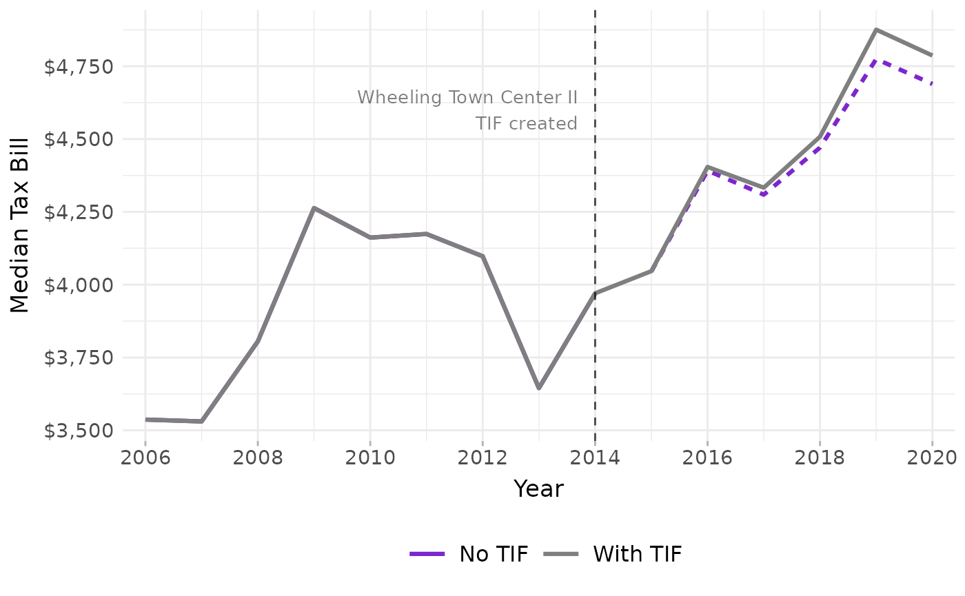
The plot shows the median tax bill for all PINs in Wheeling. The counterfactual bills are shown in purple.
The net effect of the Wheeling Town Center II TIF has been a slight increase in the median Wheeling tax bill. The effect size is small; the difference in 2020 median bills with and without the TIF is less than $100. However, when added up over many properties, this effect becomes substantial and will continue to grow if the WTC2 PINs further increase in value.
Whether or not this effect is desirable is a matter of interpretation. If the properties within the TIF would not have increased in value but for the TIF, then the TIF served its purpose, since the value it created will eventually return to the tax base. If the properties within the TIF would have increased in value regardless of the TIF, then the TIF has effectively captured part of the tax base that would otherwise have lowered rates/bills.
PTAXSIM doesn’t offer a definitive answer or make any normative claims, but it’s an incredibly useful tool for measuring these effects and weighing their potential trade-offs.
