Introduction
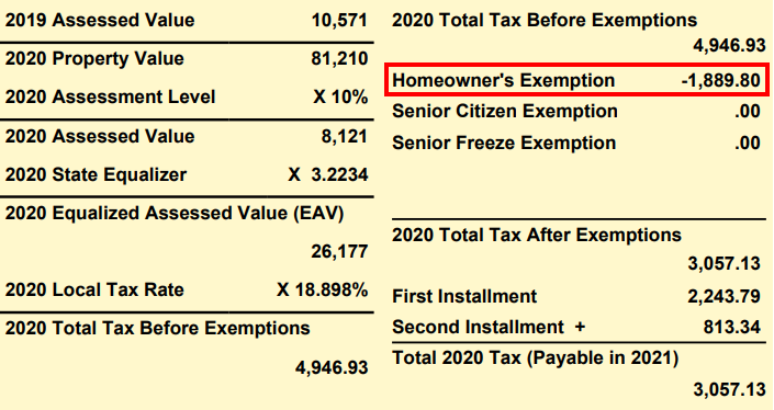
Property tax exemptions are savings that lower a homeowner’s property tax bill. They work by reducing or freezing the taxable value (Equalized Assessed Value, or EAV) of a home. For example, the most common exemption, the Homeowner Exemption, reduces EAV by $10,000.
Once the exemption EAV has been subtracted from the property’s EAV, the final EAV is multiplied by the local tax rate to get the final property tax bill. Since local tax rates can vary significantly by area, the actual effective value of each exemption likewise varies geographically.
The worth of an exemption can also be calculated directly by multiplying the local tax rate by the exemption amount. In the example bill below (PIN = 25-32-114-005-0000), the local tax rate of 18.898% is multiplied by the Homeowner Exemption flat amount of $10,000, yielding an exemption amount of $1889.80.
Exemptions affect more than just individual tax bills. Local tax rates are a ratio of the amount requested by a taxing district (the levy) to the total taxable value in that district (the base). If exemptions reduce the taxable value of property in a district, then the tax rate for that district will go up.
PTAXSIM can determine the impact of exemptions both for single properties and large areas, such as municipalities. We demonstrate both in this vignette.
Single PIN
Using PTAXSIM, let’s look at the historic impact of exemptions for a single PIN by recalculating its tax bills without any exemptions.
First, load some useful libraries and instantiate a PTAXSIM DBI
connection with the default name (ptaxsim_db_conn) expected
by PTAXSIM functions.
library(data.table)
library(dplyr)
library(here)
library(ggplot2)
library(ptaxsim)

ptaxsim_db_conn <- DBI::dbConnect(RSQLite::SQLite(), here("./ptaxsim.db"))
The PIN we’ll use is 25-32-114-005-0000, the same PIN whose bill is shown above. This is a small, single-family property in Calumet with a very typical exemption situation, just a Homeowner Exemption.
We can use the tax_bill() function to get every bill for
this PIN from the last 15 years. These bills will include any
reduction from exemptions the PIN received.
bills_w_exe <- tax_bill(2006:2020, "25321140050000", simplify = FALSE)Next, we can use dplyr to collapse the line-item bills
into totals by year.
bills_w_exe_summ <- bills_w_exe %>%
  group_by(year) %>%
  summarize(
    exe = sum(tax_amt_exe),
    bill_total = sum(final_tax_to_tif) + sum(final_tax_to_dist),
    Type = "With exemptions"
  ) %>%
  select(Year = year, Type, "Exemption Amt." = exe, "Bill Amt." = bill_total)
Finally, we can plot the change in total bill amount over time.
Click here to show plot code
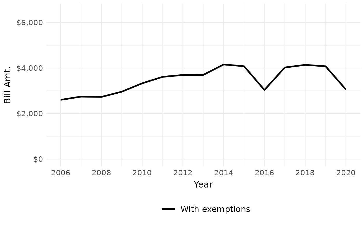
This PIN’s total tax bill has increased slightly since 2006, with some dips in the last few years. Let’s see how much it would’ve increased without its Homeowner Exemption.
Removing exemptions
We can remove exemptions by modifying the inputs to the
tax_bill() function and then recalculating each bill.
First, we retrieve the pin_dt input to
tax_bill() by using the lookup_pin() function.
This input contains all of the exemptions, AV, and EAV information for
each PIN. By default, it has the actual historical values, but we can
modify it to produce counterfactual bills. In this case, we can remove
all exemptions by setting the amount in each exemption column (prefixed
with exe_) to zero.
exe_dt <- lookup_pin(2006:2020, "25321140050000") %>%
  mutate(across(starts_with("exe_"), ~0)) %>%
  setDT(key = c("year", "pin"))
Then, we recalculate each bill using the new, zeroed-out
pin_dt.
bills_no_exe <- tax_bill(2006:2020,
  "25321140050000",
  pin_dt = exe_dt,
  simplify = FALSE
)
Next, we do the same aggregation that we did for bills with exemptions, collapsing each bill into a total by year.
bills_no_exe_summ <- bills_no_exe %>%
  group_by(year) %>%
  summarize(
    exe = sum(tax_amt_exe),
    bill_total = sum(final_tax_to_tif) + sum(final_tax_to_dist),
    Type = "No exemptions"
  ) %>%
  select(Year = year, Type, "Exemption Amt." = exe, "Bill Amt." = bill_total)
Finally, we can compare the real bills (with exemptions) to the counterfactual bills we just created (without exemptions).
Click here to show plot code
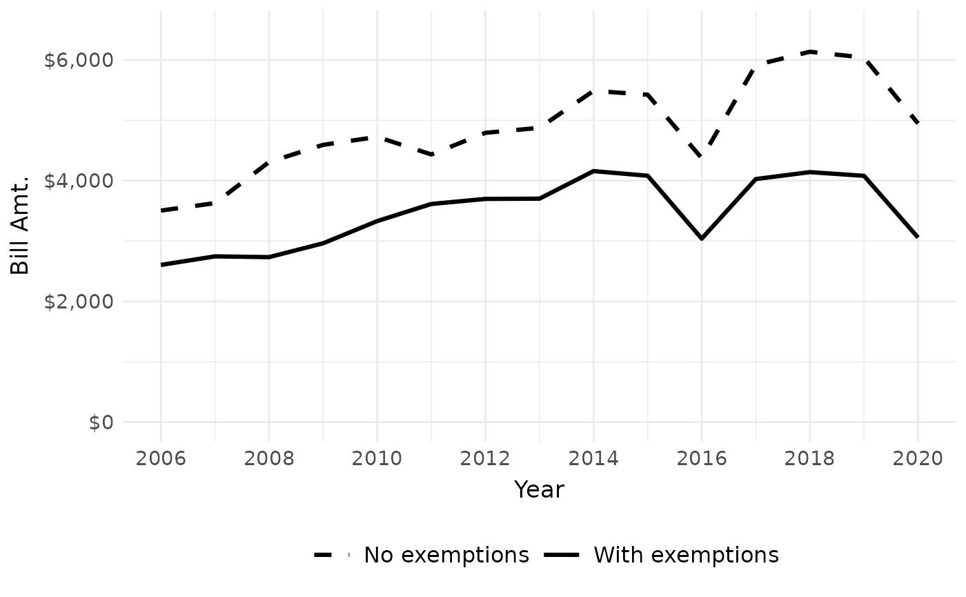
The exemption amount for this PIN has increased in tandem with increases in the local tax rate. There were also a statutory increases in the amount of the Homeowner Exemption during the same time period.
Changing exemptions
We can also use PTAXSIM to answer hypotheticals. For example, how would this PIN’s bill history change if the Homeowner Exemption increased from $10,000 to $15,000 in 2018?
To find out, we again create a modified PIN input to pass to
tax_bill(). This time, we increase the Homeowner Exemption
to $15,000 for all years after 2018.
exe_dt_2 <- lookup_pin(2006:2020, "25321140050000") %>%
  mutate(exe_homeowner = ifelse(year >= 2018, 15000, exe_homeowner)) %>%
  setDT(key = c("year", "pin"))
Then, we recalculate all the bills with the new PIN input and do the same aggregation as before.
bills_new_exe <- tax_bill(
  2006:2020,
  "25321140050000",
  pin_dt = exe_dt_2,
  simplify = FALSE
)

bills_new_exe_summ <- bills_new_exe %>%
  group_by(year) %>%
  summarize(
    exe = sum(tax_amt_exe),
    bill_total = sum(final_tax_to_tif) + sum(final_tax_to_dist),
    Type = "Changed exemption"
  ) %>%
  select(Year = year, Type, "Exemption Amt." = exe, "Bill Amt." = bill_total)
Finally, we add a third line to our plot showing the total tax bill by year after the hypothetical exemption increase in 2018.
Click here to show plot code
bills_plot_3 <- rbind(
  bills_w_exe_summ,
  bills_no_exe_summ,
  bills_new_exe_summ
) %>%
  ggplot() +
  geom_line(aes(x = Year, y = `Bill Amt.`, linetype = Type), linewidth = 1.1) +
  scale_x_continuous(n.breaks = 9) +
  scale_y_continuous(labels = scales::label_dollar(), limits = c(0, 6500)) +
  scale_linetype_manual(
    name = "",
    values = c(
      "With exemptions" = "solid",
      "No exemptions" = "dashed",
      "Changed exemption" = "dotted"
    )
  ) +
  theme_minimal() +
  theme(
    axis.title = element_text(size = 13),
    axis.title.x = element_text(margin = margin(t = 6)),
    axis.title.y = element_text(margin = margin(r = 6)),
    axis.text = element_text(size = 11),
    strip.text = element_text(size = 16),
    strip.background = element_rect(fill = "#c9c9c9"),
    legend.title = element_text(size = 14),
    legend.key.size = unit(24, "points"),
    legend.text = element_text(size = 12),
    legend.position = "bottom"
  )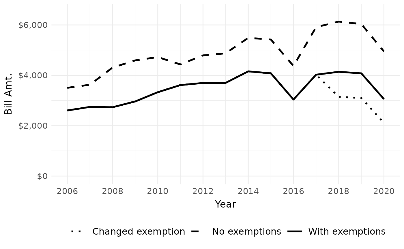
Increasing the Homeowner Exemption to $15,000 would save this property owner around $1,000 per year in taxes. However, this hypothetical does not account for changes in the tax base that would occur if overall exemption amounts changed, so it is (slightly) inaccurate.
Many PINs
PTAXSIM can also perform more complex analysis, such as measuring the
impact of exemptions in a given area. To perform this analysis, we can
again use the tax_bill() function to calculate tax bills
before and after exemptions are removed, this time for many PINs.
Removing exemptions
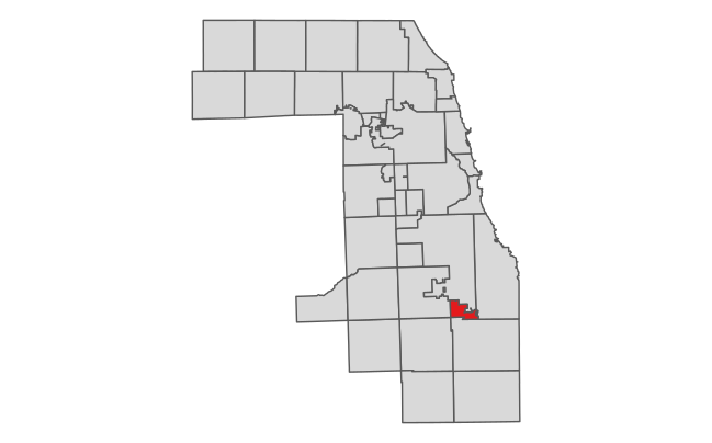
Let’s look at the overall effect of exemptions in the Cook County township of Calumet, shown in red below.
First, we can use the PTAXSIM database to get a list of all the unique PINs in Calumet township. We can also create a vector of years we’re interested in.
t_pins <- DBI::dbGetQuery(
  ptaxsim_db_conn,
  "
  SELECT DISTINCT pin
  FROM pin
  WHERE substr(tax_code_num, 1, 2) = '14'
  "
)
t_pins <- t_pins$pin
t_years <- 2006:2020
Next, we can generate bills for all PINs in Calumet for the past 15 years. These bills will include any exemptions they actually received.
We’re using data.table syntax here because it’s much
faster than dplyr when working with large data. Note that
PTAXSIM functions always output a data.table with keys.
t_bills_w_exe <- tax_bill(t_years, t_pins)[, stage := "With exemptions"]Unlike a single PIN, removing exemptions from many PINs means that the base (the amount of total taxable value available) will change substantially. In order to accurately model the effect of removing exemptions, we need to fully recalculate the base of each district by adding the sum of taxable value recovered from each PIN.
To start, we use the lookup_pin() function to recover
the total EAV of exemptions for each PIN.
t_pin_dt_no_exe <- lookup_pin(t_years, t_pins)
t_pin_dt_no_exe[, tax_code := lookup_tax_code(year, pin)]

exe_cols <- names(t_pin_dt_no_exe)[startsWith(names(t_pin_dt_no_exe), "exe_")]
t_tc_sum_no_exe <- t_pin_dt_no_exe[,
  .(exe_total = sum(rowSums(.SD))),
  .SDcols = exe_cols,
  by = .(year, tax_code)
]
Next, we recalculate the base of all taxing districts in Calumet by adding the EAV returned from exemptions to each district’s total EAV.
t_agency_dt_no_exe <- lookup_agency(t_years, t_pin_dt_no_exe$tax_code)
t_agency_dt_no_exe[
  t_tc_sum_no_exe,
  on = .(year, tax_code),
  agency_total_eav := agency_total_eav + exe_total
]
Then, we again alter the pin_dt input by setting all
exemption columns equal to zero.
t_pin_dt_no_exe[, (exe_cols) := 0][, c("tax_code") := NULL]We recalculate all Calumet tax bills without exemptions and
with an updated tax base for each district (passed via
agency_dt).
t_bills_no_exe <- tax_bill(
  year_vec = t_years,
  pin_vec = t_pins,
  agency_dt = t_agency_dt_no_exe,
  pin_dt = t_pin_dt_no_exe
)[
  , stage := "No exemptions"
]
To see the results, we can calculate the average tax bill by year by property type (residential or commercial), with and without exemptions. We can also index the result to the earliest year available (in this case 2006) to make the different property types comparable on the same scale.
# Little function to get the statistical mode
Mode <- function(x) {
  ux <- unique(x)
  ux[which.max(tabulate(match(x, ux)))]
}

t_no_exe_summ <- rbind(t_bills_w_exe, t_bills_no_exe)[
  , class := Mode(substr(class, 1, 1)),
  by = pin
][
  class %in% c("2", "3", "5"),
][
  , class := ifelse(class == "2", "Residential", "Commercial")
][
  , .(total_bill = sum(final_tax)),
  by = .(year, pin, class, stage)
][
  , .(avg_bill = mean(total_bill)),
  by = .(year, class, stage)
][
  , idx_bill := (avg_bill / avg_bill[year == 2006]) * 100,
  by = .(class, stage)
]
Finally, we can plot the average bill with and without exemptions by property type.
Click here to show plot code
t_annot <- tibble(
  class = c("Residential", "Commercial"),
  x = c(2008, 2006.4),
  y = c(105, 115)
)

# Plot the change in indexed values over time
t_no_exe_summ_plot <- ggplot(data = t_no_exe_summ) +
  geom_line(
    aes(x = year, y = idx_bill, color = class, linetype = stage),
    linewidth = 1.1
  ) +
  geom_text(
    data = t_annot,
    aes(x = x, y = y, color = class, label = class),
    hjust = 0
  ) +
  scale_y_continuous(name = "Average Tax Bill, Indexed to 2006") +
  scale_x_continuous(name = "Year", n.breaks = 10, limits = c(2006, 2020.4)) +
  scale_linetype_manual(
    name = "",
    values = c("With exemptions" = "solid", "No exemptions" = "dashed")
  ) +
  scale_color_brewer(name = "", palette = "Set1", direction = -1) +
  guides(color = "none") +
  facet_wrap(vars(class)) +
  theme_minimal() +
  theme(
    axis.title = element_text(size = 13),
    axis.title.x = element_text(margin = margin(t = 6)),
    axis.title.y = element_text(margin = margin(r = 6)),
    axis.text.y = element_text(size = 11),
    strip.text = element_text(size = 16),
    strip.background = element_rect(fill = "#c9c9c9"),
    legend.title = element_text(size = 14),
    legend.key.size = unit(24, "points"),
    legend.text = element_text(size = 12),
    legend.position = "bottom"
  )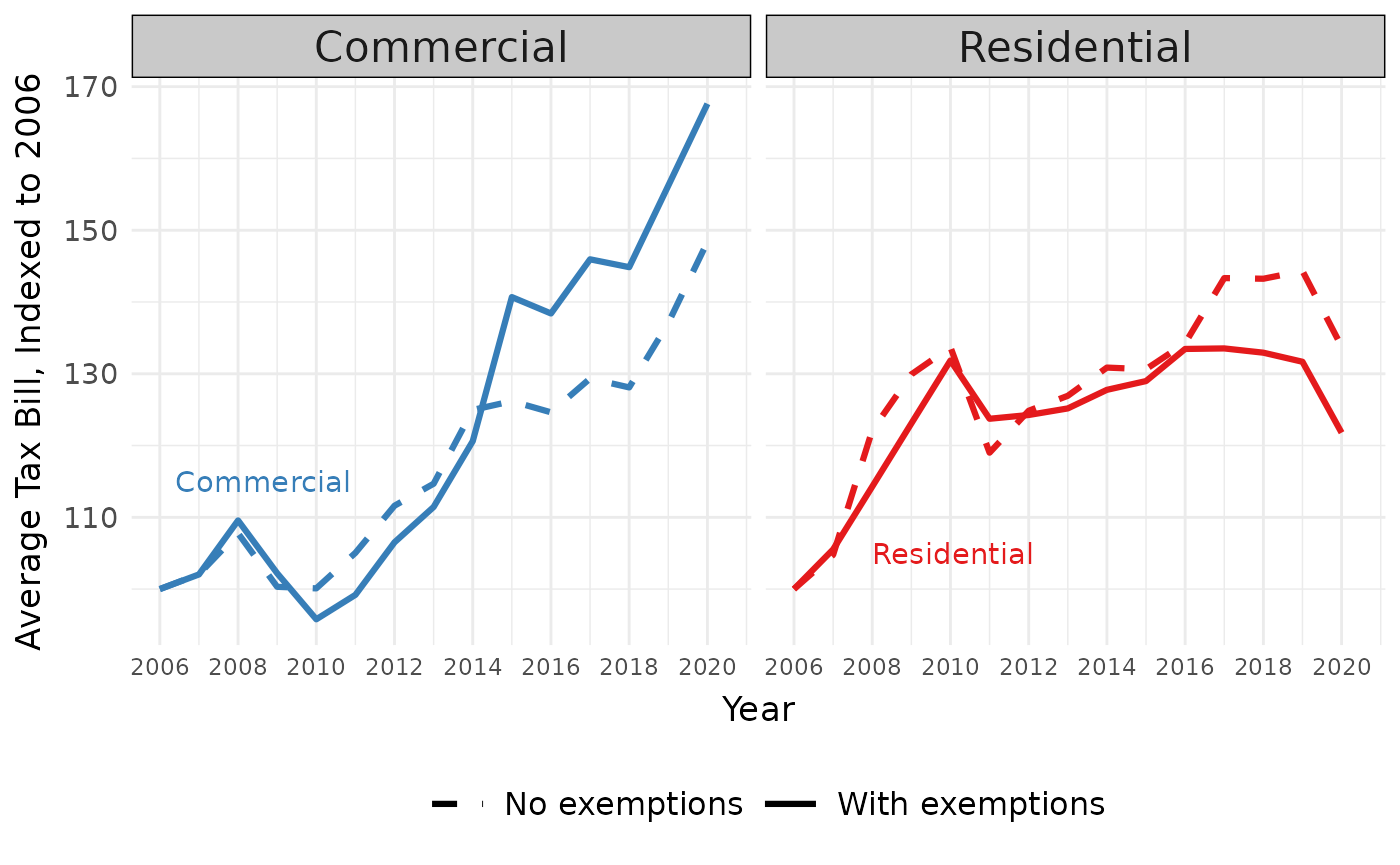
Exemptions in Calumet have significantly increased in both volume and amount (via increased tax rates) in recent years. In 2019, the average residential homeowner saved around $1,100 via exemptions.
Conversely, Calumet’s commercial property owners have picked up an increasingly large share of the overall tax burden since 2006. In 2019, the average commercial property paid about $1,100 more than they would have if exemptions did not exist.
Changing exemptions
PTAXSIM can also answer hypotheticals about large areas. For example, how would the average residential tax bill in Calumet change if the Senior Exemption increased by $5,000 and the Senior Freeze Exemption was removed?
To find out, we again create a PIN input with modified exemption amounts, then recalculate the base by taking the difference between the real and hypothetical exemptions.
t_pin_dt_new_exe <- lookup_pin(t_years, t_pins)
t_pin_dt_new_exe[, tax_code := lookup_tax_code(year, pin)]

t_tc_sum_new_exe <- t_pin_dt_new_exe[
  , .(exe_total = sum(exe_freeze - (5000 * (exe_senior != 0)))),
  by = .(year, tax_code)
]
Next, we recalculate the base of each district. This time, the base may lose some EAV, since the Senior Exemption is increasing substantially.
t_agency_dt_new_exe <- lookup_agency(t_years, t_pin_dt_new_exe$tax_code)
t_agency_dt_new_exe[
  t_tc_sum_new_exe,
  on = .(year, tax_code),
  agency_total_eav := agency_total_eav + exe_total
]
Then, we again alter the pin_dt input by setting the
Senior Freeze Exemption to zero and adding $5,000 to any Senior
Exemption.
t_pin_dt_new_exe <- t_pin_dt_new_exe[
  , exe_freeze := 0
][
  exe_senior != 0, exe_senior := exe_senior + 5000
][
  , c("tax_code") := NULL
]
We again recalculate all Calumet tax bills with our updated exemptions and with an updated tax base for each district.
t_bills_new_exe <- tax_bill(
  year_vec = t_years,
  pin_vec = t_pins,
  agency_dt = t_agency_dt_new_exe,
  pin_dt = t_pin_dt_new_exe
)[
  , stage := "Changed exemptions"
]
Then, do the same aggregation and indexing we did previously, this time using the updated bills.
t_new_exe_summ <- rbind(t_bills_w_exe, t_bills_new_exe)[
  , class := Mode(substr(class, 1, 1)),
  by = pin
][
  class %in% c("2", "3", "5"),
][
  , class := ifelse(class == "2", "Residential", "Commercial")
][
  , .(total_bill = sum(final_tax)),
  by = .(year, pin, class, stage)
][
  , .(avg_bill = mean(total_bill)),
  by = .(year, class, stage)
][
  , idx_bill := (avg_bill / avg_bill[year == 2006]) * 100,
  by = .(class, stage)
]
Finally, we can plot the original bills against the updated ones.
Click here to show plot code
t_new_exe_summ_plot <- ggplot(data = t_new_exe_summ) +
  geom_line(
    aes(x = year, y = idx_bill, color = class, linetype = stage),
    linewidth = 1.1
  ) +
  geom_text(
    data = t_annot,
    aes(x = x, y = y, color = class, label = class),
    hjust = 0
  ) +
  scale_y_continuous(name = "Average Tax Bill, Indexed to 2006") +
  scale_x_continuous(name = "Year", n.breaks = 10, limits = c(2006, 2020.4)) +
  scale_linetype_manual(
    name = "",
    values = c("With exemptions" = "solid", "Changed exemptions" = "dotted")
  ) +
  scale_color_brewer(name = "", palette = "Set1", direction = -1) +
  guides(color = "none") +
  facet_wrap(vars(class)) +
  theme_minimal() +
  theme(
    axis.title = element_text(size = 13),
    axis.title.x = element_text(margin = margin(t = 6)),
    axis.title.y = element_text(margin = margin(r = 6)),
    axis.text.y = element_text(size = 11),
    strip.text = element_text(size = 16),
    strip.background = element_rect(fill = "#c9c9c9"),
    legend.title = element_text(size = 14),
    legend.key.size = unit(24, "points"),
    legend.text = element_text(size = 12),
    legend.position = "bottom"
  )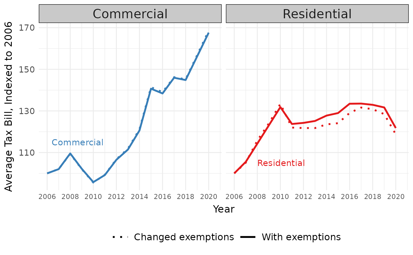
The net effect of increasing the Senior Exemption while removing the Senior Freeze Exemption is a slight decrease in the average bill. However, this conclusion is ambiguous, complicated by the fact that the Senior Freeze is means-tested, while the Senior Exemption is not. The “real-world effect” of our hypothetical policy change would most likely be an increase in the property tax bills of poorer seniors, even though the average bill decreased.
Ultimately, with some careful coding and assumptions, PTAXSIM (and its included data) can be used to test almost any hypothetical change in exemptions.
