Measuring the impact of appeals • ptaxsim

Introduction

Appeals are a way to contest the assessed value (AV) of a property after it is determined by the Assessor’s Office. If an appeal is granted, the property value is lowered and the owner pays taxes on the reduced value. Cook County has three opportunities to appeal, which happen in order:

Assessor’s Office
Board of Review
Property Tax Appeal Board (PTAB) or Circuit Court

Due to the nature of Cook County’s property tax system, appeals are a zero-sum affair: each successful appeal with the Assessor’s Office or Board of Review will increase the property tax bill of other property owners. However, measuring this effect is difficult since it requires recalculating tax bills pre- and post-appeal for many properties.

Enter PTAXSIM, which can simulate counterfactual estimated tax bills and contains data on assessed values at each “stage” of appeals. The stages are stored in separate columns of the pin table in the PTAXSIM database:

av_mailed - Initial assessed values when mailed to property owners, after Desk Review
av_certified - Assessed values after Assessor’s Office appeals
av_board - Assessed values after Board of Review appeals
av_clerk - Final assessed values used by the Clerk and Treasurer to calculate bills. Identical to av_board in 99.9% of cases

We can use these values and PTAXSIM’s tax_bill() function to calculate pre- and post-appeal estimated property tax bills and ultimately determine the impact of appeals. This vignette will cover that process.

Appeals in Chicago

Using PTAXSIM, we’re going to examine property values and tax bills in Chicago after its 2024 reassessment.

First, load some useful libraries and instantiate a PTAXSIM database connection with the default name (ptaxsim_db_conn) expected by PTAXSIM functions.

library(DBI)
library(data.table)
library(dplyr)
library(ggplot2)
library(ggspatial)
library(glue)
library(here)
library(purrr)
library(ptaxsim)
library(sf)

ptaxsim_db_conn <- DBI::dbConnect(RSQLite::SQLite(), here("./ptaxsim.db"))

Gathering PINs of interest

To determine the impact of appeals, we first need a way to gather all the properties (PINs) in Chicago. Fortunately, PTAXSIM’s database has all the data required to accomplish this task.

First, we’ll need to determine the City of Chicago’s agency number. This is the ID used by the Clerk to track different taxing bodies. To find Chicago’s ID, we can directly query PTAXSIM’s database and look in the agency_info table:

chi_agency_nums <- DBI::dbGetQuery(
  ptaxsim_db_conn,
  "SELECT agency_num, agency_name
  FROM agency_info
  WHERE agency_name LIKE '%CITY OF CHICAGO%'"
)

head(chi_agency_nums)
#>   agency_num                            agency_name
#> 1  030210000                        CITY OF CHICAGO
#> 2  030210001           CITY OF CHICAGO LIBRARY FUND
#> 3  030210002 CITY OF CHICAGO SCHOOL BLDG & IMP FUND
#> 4  030210100 CITY OF CHICAGO SPECIAL SERVICE AREA 1
#> 5  030210101 CITY OF CHICAGO SPECIAL SERVICE AREA 2
#> 6  030210102 CITY OF CHICAGO SPECIAL SERVICE AREA 3

Here we can see the various taxing bodies associated with the City of Chicago. The agency number we want is 030210000 for the municipality, CITY OF CHICAGO. With the agency number, we can find all of the tax codes that make up the municipality. To do so, we can again query PTAXSIM directly, this time looking in the tax_code table:

chi_tax_codes <- DBI::dbGetQuery(
  ptaxsim_db_conn, "
  SELECT tax_code_num
  FROM tax_code
  WHERE agency_num = '030210000'
  AND year = 2024
  "
)

Finally, we can find all of Chicago’s PINs with one last direct query. This time we’ll look in the pin table using the tax codes that make up Chicago. We’ll use the glue library for string expansion to make things a bit easier:

chi_pins <- DBI::dbGetQuery(
  ptaxsim_db_conn,
  glue_sql("
    SELECT pin, class,
    av_certified,
    av_board
    FROM pin
    WHERE tax_code_num IN ({chi_tax_codes$tax_code_num*})
    AND pin.year = 2024
    ",
    .con = ptaxsim_db_conn
  )
)

chi_tif_pins <- DBI::dbGetQuery(
  ptaxsim_db_conn,
  glue_sql("
    SELECT pin,
    agency_num,
    pin_eav,
    pin_frozen_eav
    FROM pin_tif_distribution
    WHERE tax_code_num IN ({chi_tax_codes$tax_code_num*})
    and year = 2024
    ",
    .con = ptaxsim_db_conn
  )
)

chi_pins <- chi_pins %>%
  left_join(chi_tif_pins)

Mapping Chicago

We can query the pin_geometry table from PTAXSIM’s SQLite database or use the use the `lookup_pin10() function in order to map Chicago’s parcels by their major class codes.

Mapping all Chicago parcels is a memory intensive job, so we created the map with a simple python script which has proven to be more efficient at mapping large quantities of data. That code can be viewed below.

Click here to show plot code

import sqlite3
import pandas as pd
import geopandas as gpd
from shapely import wkt
from pathlib import Path
import contextily as ctx
import matplotlib.pyplot as plt
import matplotlib.patches as mpatches
from matplotlib_scalebar.scalebar import ScaleBar

DB_PATH = "/home/user/ptaxsim-2024.0.0.db"
TAX_YEAR = 2024
TAX_CODE_PREFIXES = ["70", "71", "72", "73", "74", "75", "76", "77"]
OUTPUT_DIR = Path("/home/user/output")
OUTPUT_DIR.mkdir(exist_ok=True)

def classify_property(class_code):
    if pd.isna(class_code):
        return "Other"
    first = str(class_code).strip()[0]
    return {
        "0": "Other",
        "1": "Other",
        "2": "Residential",
        "3": "Commercial",
        "4": "Other",
        "5": "Commercial",
        "6": "Other",
        "7": "Other",
        "8": "Other",
        "9": "Other"
    }.get(first, "Other")

color_map = {
    "Residential": "#29428D",
    "Commercial": "#FFAF00",
    "Other": "#787878"
}

conn = sqlite3.connect(DB_PATH)
prefix_list = "','".join(TAX_CODE_PREFIXES)

print("Loading PINs...")
pins = pd.read_sql(f"""
    SELECT pin, tax_code_num, class
    FROM pin
    WHERE year = {TAX_YEAR}
    AND substr(tax_code_num, 1, 2) IN ('{prefix_list}')
""", conn)
pins["pin10"] = pins["pin"].str[:10]
pins["property_type"] = pins["class"].apply(classify_property)

# Deduplicate to one row per pin10
pins_deduped = pins.groupby("pin10").agg(
    property_type=("property_type", "first")
).reset_index()

print("Loading geometries...")
pin10_list = "','".join(pins["pin10"].unique())
geo = pd.read_sql(f"""
    SELECT pin10, geometry
    FROM pin_geometry_raw
    WHERE pin10 IN ('{pin10_list}')
    AND start_year <= {TAX_YEAR}
    AND end_year >= {TAX_YEAR}
""", conn)
conn.close()

merged = geo.merge(pins_deduped, on="pin10", how="inner")
merged["geometry"] = merged["geometry"].apply(wkt.loads)
gdf = gpd.GeoDataFrame(merged, geometry="geometry", crs="EPSG:4326")
gdf["geometry"] = gdf.geometry.buffer(0)

# Reproject to Illinois State Plane for accurate scale bar
gdf = gdf.to_crs("EPSG:26971")

# Fix invalid geometries again after reprojection
gdf["geometry"] = gdf.geometry.buffer(0)

# Township boundary outline
boundary = gdf.dissolve().boundary

# Map each parcel to its color
gdf["color"] = gdf["property_type"].map(color_map)

print("Plotting...")
# Get the aspect ratio from your data bounds
minx, miny, maxx, maxy = gdf.total_bounds
aspect = (maxy - miny) / (maxx - minx)
fig_width = 12
fig_height = fig_width * aspect

fig, ax = plt.subplots(1, 1, figsize=(fig_width, fig_height))

# Plot each property type separately so legend works cleanly
for ptype, color in color_map.items():
    subset = gdf[gdf["property_type"] == ptype]
    if len(subset) > 0:
        subset.plot(ax=ax, color=color, linewidth=0.1, edgecolor=color, alpha=0.8)

# Township boundary
boundary.plot(ax=ax, color="black", linewidth=0.06)

# Add background basemap to the image
ctx.add_basemap(
    ax,
    crs=gdf.crs.to_string(),
    source=ctx.providers.CartoDB.Positron,
    alpha=0.5
)

# Legend
patches = [mpatches.Patch(color=color, label=ptype) for ptype, color in color_map.items()]
ax.legend(handles=patches, loc="lower center", ncol=3, fontsize=11,
          bbox_to_anchor=(0.5, -0.03), frameon=False, markerscale=2)

# Remove axis labels 
ax.set_axis_off()

# Save map to specified path
out_path = OUTPUT_DIR / f"map_property_types_static_{TAX_YEAR}.png"
plt.savefig(out_path, dpi=150, bbox_inches="tight", pad_inches=0)
print(f"Saved {out_path}")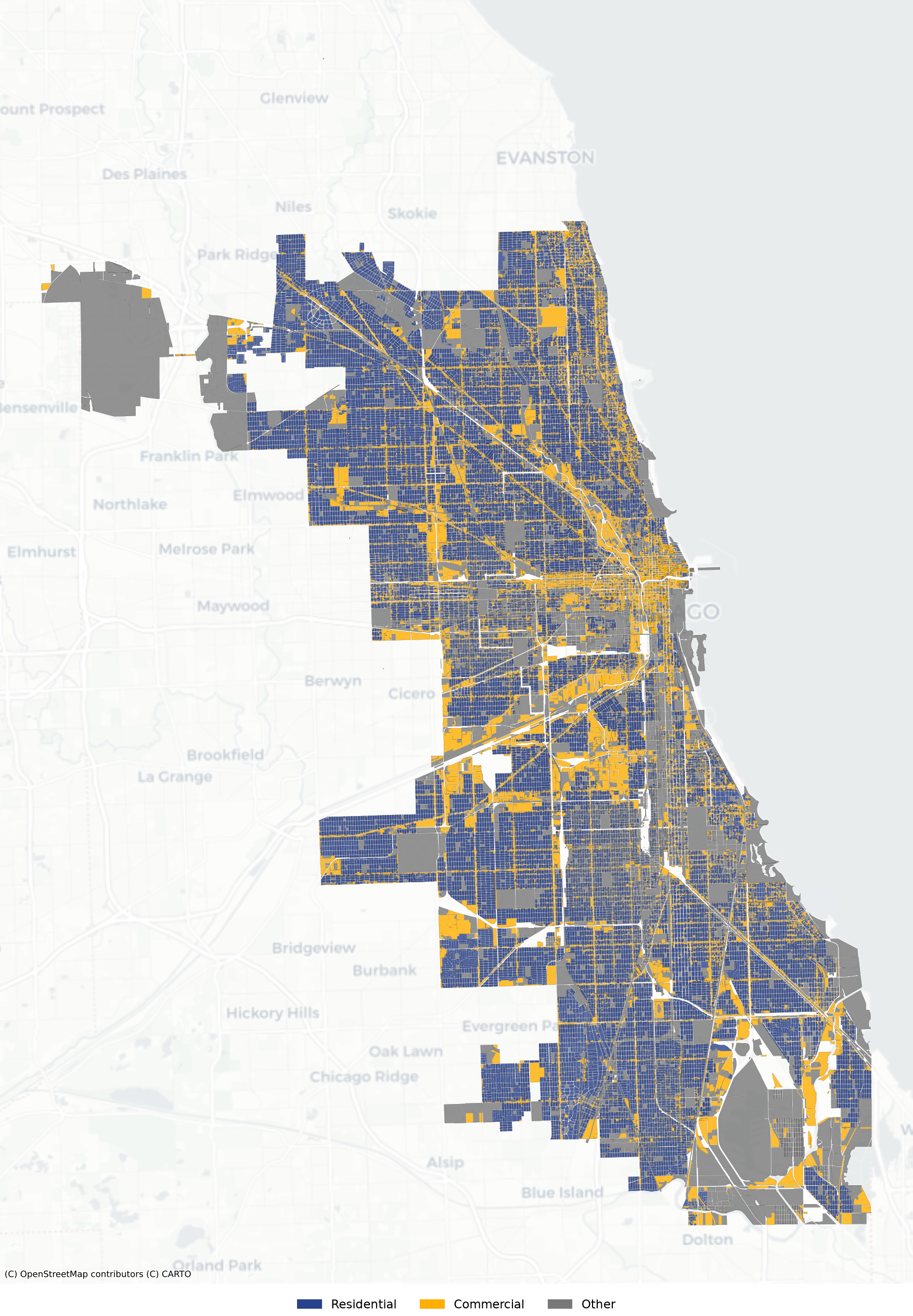

The map illustrates that geographically, most of Chicago’s parcels are residential, with commercial and other property classes concentrated downtown and along various commercial corridors.

Appeals’ impact on AVs

Now that we’ve gathered our PINs of interest, we can start to investigate how they were affected by appeals after the 2024 reassessment. Let’s start by looking at changes in assessed values. We can gather the AVs from each assessment stage using PTAXSIM’s lookup_pin() function.

# Iterate through the difference stages, then combine into a single data.frame
chi_pins_all <- purrr::map_dfr(c("mailed", "certified", "board"), function(x) {
  lookup_pin(2024, chi_pins$pin, stage = x) %>%
    mutate(stage = x)
})

# Append 2023 final values to use as a starting point for an index
chi_pins_all <- lookup_pin(2023, chi_pins$pin, stage = "board") %>%
  mutate(stage = "board") %>%
  bind_rows(chi_pins_all)

Next, we get the median AV for each assessment stage and major class. We also calculate the percent change in median AV compared to the 2023 board stage, meaning a value of 25% indicates the median AV has increased relative to the 2023 board median AV.

chi_pins_summ <- chi_pins_all %>%
  mutate(major_class = substr(class, 1, 1)) %>%
  filter(major_class %in% c("2", "3", "5")) %>%
  mutate(
    major_class = recode_factor(
      major_class,
      "2" = "2 - Residential",
      "3" = "3 & 5 - Commercial",
      "5" = "3 & 5 - Commercial"
    )
  ) %>%
  group_by(year, stage, major_class) %>%
  summarize(med_av = median(av), count = n()) %>%
  ungroup() %>%
  mutate(
    stage = factor(
      paste0(year, "\n", stage),
      levels = c(
        "2023\nboard", "2024\nmailed",
        "2024\ncertified", "2024\nboard"
      )
    ),
    perc_change = (med_av - med_av[stage == "2023\nboard"]) /
      med_av[stage == "2023\nboard"] * 100
  )

Finally, we can plot the percent change in median AV over time to see how reassessment and the subsequent appeals at each stage impacted assessed values.

Click here to show plot code

# Create conditional x-axis colors for reassessment stage
stage_labs <- ifelse(
  as.factor(c(
    "2023\nboard", "2024\nmailed",
    "2024\ncertified", "2024\nboard"
  )) == "2024\nmailed",
  "red", "black"
)

chi_pins_av_plot <- ggplot() +
  geom_vline(
    xintercept = "2024\nmailed",
    linetype = "dotted",
    color = "red"
  ) +
  geom_line(
    data = chi_pins_summ,
    aes(x = stage, y = perc_change, color = major_class, group = major_class),
    linewidth = 1.1
  ) +
  scale_color_manual(name = "", values = c("#29428d", "#ffaf00")) +
  scale_y_continuous(
    limits = c(0, 50),
    labels = scales::label_percent(scale = 1)
  ) +
  labs(
    x = "Stage",
    y = NULL,
    title = "Median AV percent change relative to 2023 Board",
    caption = "Highlighted stage is a reassessment"
  ) +
  theme_minimal() +
  theme(
    axis.title = element_text(size = 13),
    axis.title.x = element_text(margin = margin(t = 6)),
    axis.title.y = element_text(margin = margin(r = 6), size = 12),
    axis.text = element_text(size = 11),
    axis.text.x = element_text(color = stage_labs),
    strip.text = element_text(size = 16),
    strip.background = element_rect(fill = "#c9c9c9"),
    legend.title = element_text(size = 14),
    legend.key.size = unit(24, "points"),
    legend.text = element_text(size = 12),
    legend.position = "right"
  )

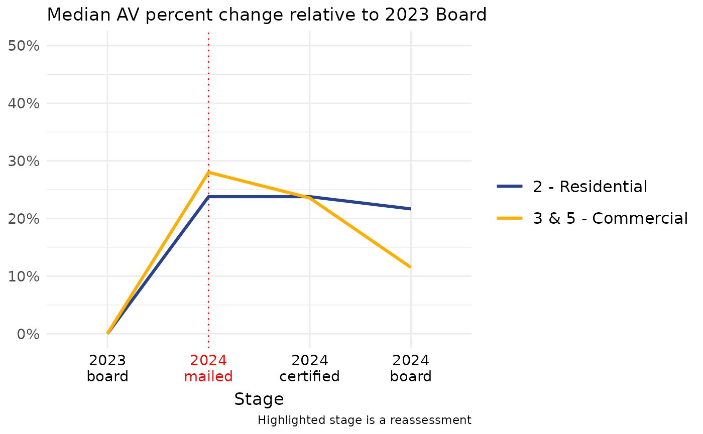
There’s a significant drop in the median commercial property AV due to appeals, particularly after the second level of review (at the Board of Review). However, commercial properties also received larger AV increases during the 2024 reassessment compared to residential properties.

Appeals’ impact on bills

Now that we’ve looked at AVs, we can also use PTAXSIM to examine the impact of appeals on tax bills. To do so, we’ll first calculate bills at each stage of assessment. The bills for the mailed and certified stages are counterfactual; they represent estimates of what bills would have been at each stage if no further appeals were granted. The board stage bills are the actual bills received by property owners.

# Calculate tax bills from 2024 at each stage of appeal. Note that recalculating
# bills with counterfactual AVs also requires recalculating the base of each
# taxing district
chi_bills_all <- purrr::map_dfr(c("mailed", "certified", "board"), function(x) {
  chi_pin_dt_actual <- lookup_pin(2024, chi_pins$pin, stage = "clerk")
  chi_pin_dt_stage <- lookup_pin(
    2024,
    chi_pins$pin,
    stage = x
  )

  # We need to calculate the new taxable EAV for each PIN at the various
  # stages. Changes to AV impacts the TIF share for PINs in TIFs, as well
  # as the senior freeze exemption amount for PINs with that exemption.

  # The base of each district in the included PTAXSIM data is based on 2024
  # board (post-appeal) values. It is therefore smaller than it would be if
  # appeals had not been granted. As such, we need to calculate the difference
  # for each PIN between the AV at each stage and the AV at the board stage,
  # then add the total difference to each district's base
  chi_pin_diff <- chi_pin_dt_actual %>%
    left_join(
      chi_pin_dt_stage %>%
        select(year, pin, stage_eav = eav),
      by = c("year", "pin")
    ) %>%
    left_join(chi_pins) %>%
    mutate(
      tax_code = lookup_tax_code(2024, pin),
      exe_total = rowSums(across(starts_with("exe_"))),
      # We want to first calculate taxable EAV which is EAV minus exemptions.
      # The stage taxable EAV should be the same as the actual taxable EAV
      # if the PIN received a senior freeze exemption
      taxable_eav = eav - exe_total,
      taxable_stage_eav = ifelse(
        exe_freeze > 0,
        eav - exe_total,
        stage_eav - exe_total
      ),
      # We need to consider if a PIN is in a TIF to determine if any pre-appeal
      # EAV will be added to the tax base or diverted to the TIF increment
      eav_diff = case_when(
        # Scenario 1: If both stage and actual EAV exceed the PIN's frozen EAV
        # then the extra pre-appeal reduction EAV gets diverted to the TIF
        taxable_eav > pin_frozen_eav &
          taxable_stage_eav > pin_frozen_eav ~ 0,
        # Scenario 2: If the actual EAV is less than the frozen EAV and
        # pre-appeal stage EAV is greater than frozen EAV, the diff between
        # actual EAV and frozen EAV is added into the tax base
        taxable_eav < pin_frozen_eav &
          taxable_stage_eav > pin_frozen_eav ~ pin_frozen_eav - taxable_eav,
        # Scenario 3: If the pre-appeal stage is less than the frozen EAV
        # all of the EAV diff is added to the tax base.
        pin_frozen_eav > taxable_stage_eav ~ taxable_stage_eav - taxable_eav,
        # For all of the non-TIF PINs, calculate the EAV diff
        TRUE ~ taxable_stage_eav - taxable_eav
      ),
      pin_stage_increment = ifelse(
        pin_frozen_eav < taxable_stage_eav,
        taxable_stage_eav - pin_frozen_eav,
        0
      )
    )

  # Calculate each TIF PIN's TIF share for the stages
  tif_stage_share <- chi_pin_diff %>%
    mutate(tif_pin_share = pin_stage_increment / taxable_stage_eav) %>%
    select(pin, tif_pin_share)

  # Aggregate the EAV diff by tax code which will enable joining to
  # tax district data
  chi_tax_code_diff <- chi_pin_diff %>%
    group_by(year, tax_code) %>%
    summarize(
      eav_diff_total = sum(eav_diff),
    )

  # Update each district base using the amount recovered from "undoing" appeals
  chi_agency_dt <- lookup_agency(chi_pin_diff$year, chi_pin_diff$tax_code) %>%
    left_join(chi_tax_code_diff, by = c("year", "tax_code")) %>%
    # Aggregate the total differences for each district
    group_by(agency_num, agency_name) %>%
    mutate(
      eav_diff_total = sum(eav_diff_total)
    ) %>%
    ungroup() %>%
    mutate(
      agency_total_eav = agency_total_eav + eav_diff_total
    ) %>%
    select(
      -eav_diff_total
    ) %>%
    as.data.table() %>%
    setkey(year, tax_code, agency_num)

  tax_bill(
    2024,
    chi_pin_dt_stage$pin,
    pin_dt = chi_pin_dt_stage,
    agency_dt = chi_agency_dt
  ) %>%
    mutate(stage = x)
})

# Append unaltered 2023 bills, again as a starting point for our index
chi_bills_all <- tax_bill(2023, chi_pins$pin) %>%
  mutate(stage = "board") %>%
  bind_rows(chi_bills_all)

We now have two sets of bills: the real bills from each board stage, and the counterfactual bills from the mailed and certified stages. Each bill from tax_bill() is broken out into per-district line items. In order to visualize the changes in bills, we first collapse the bills into their totals, then aggregate and index them in the same way we did for AVs.

chi_bills_summ <- chi_bills_all %>%
  group_by(year, pin, class, stage) %>%
  summarize(bill_total = sum(final_tax)) %>%
  ungroup() %>%
  mutate(major_class = substr(class, 1, 1)) %>%
  filter(major_class %in% c("2", "3", "5")) %>%
  mutate(
    major_class = recode_factor(
      major_class,
      "2" = "2 - Residential",
      "3" = "3 & 5 - Commercial",
      "5" = "3 & 5 - Commercial"
    )
  ) %>%
  group_by(year, stage, major_class) %>%
  summarize(med_bill = median(bill_total), count = n()) %>%
  ungroup() %>%
  mutate(
    stage = factor(
      paste0(year, "\n", stage),
      levels = c(
        "2023\nboard", "2024\nmailed",
        "2024\ncertified", "2024\nboard"
      )
    ),
    perc_change = (med_bill - med_bill[stage == "2023\nboard"]) /
      med_bill[stage == "2023\nboard"] * 100
  )

We can then plot the percent change in the median total tax bill (indexed to the 2023 board median bill) to see the effect of each stage of appeals. The earlier plot showing assessed values is added for reference.

Click here to show plot code

chi_bills_plot <- bind_rows(
  chi_pins_summ %>% mutate(type = "Assessed Values"),
  chi_bills_summ %>% mutate(type = "Tax Bills")
) %>%
  ggplot() +
  geom_vline(
    xintercept = "2024\nmailed",
    linetype = "dotted",
    color = "red"
  ) +
  geom_line(
    aes(x = stage, y = perc_change, color = major_class, group = major_class),
    linewidth = 1.1
  ) +
  scale_color_manual(name = "", values = c("#29428d", "#ffaf00")) +
  scale_y_continuous(
    limits = c(0, 50),
    labels = scales::label_percent(scale = 1)
  ) +
  labs(
    x = "Stage",
    y = "Median Value, Indexed to 2023 Board",
    caption = "Highlighted stage is a reassessment"
  ) +
  facet_wrap(vars(type)) +
  theme_minimal() +
  theme(
    axis.title = element_text(size = 13),
    axis.title.x = element_text(margin = margin(t = 6)),
    axis.title.y = element_text(margin = margin(r = 6), size = 12),
    axis.text = element_text(size = 11),
    axis.text.x = element_text(color = stage_labs),
    strip.text = element_text(size = 16),
    legend.title = element_text(size = 14),
    legend.key.size = unit(24, "points"),
    legend.text = element_text(size = 12),
    legend.position = "bottom"
  )

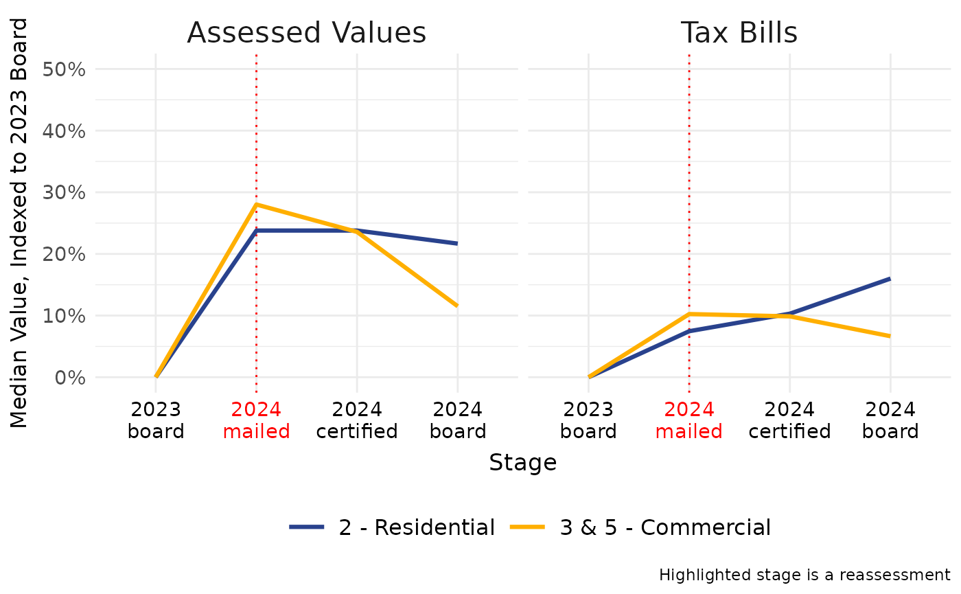
Overall, post-reassessment appeals in Chicago resulted in a roughly 9% increase in the median residential tax bill and a 5% decrease in the median commercial tax bill. Without appeals, particularly at the Board of Review, the median commercial bill would have increased roughly 10% from 2023.

Counterfactual scenario

The plot above shows the zero-sum nature of assessment appeals. The large AV decreases for commercial properties in Chicago raised the median tax bill for residential property owners. We can test this by holding the assessed value of all commercial properties constant (as if no appeals were granted) and then recalculating tax bills.

# Again we need to calculate bills at each stage of appeal. This time it's more
# complicated since we need to exclude commercial appeals
chi_cntr_all <- purrr::map_dfr(c("mailed", "certified", "board"), function(x) {
  chi_pin_dt_actual <- lookup_pin(2024, chi_pins$pin, stage = "clerk")
  chi_pin_dt_mailed <- lookup_pin(
    2024,
    chi_pins$pin,
    stage = "mailed",
  )
  chi_pin_dt_stage <- lookup_pin(
    2024,
    chi_pins$pin,
    stage = x
  )

  # To recalculate the base, we get two distinct sets of differences:
  # 1. Residential PINs act normally, the amount back to the base from each
  #    PIN is the difference between the stage EAV and the 2024 final EAV
  # 2. Commercial PINs are not granted appeals. So the amount back to the base
  #    for all stages is the difference between the initial mailed value (no
  #    appeals) and the final 2024 value (which contains appeals)
  chi_pin_diff <- rbind(
    chi_pin_dt_actual %>%
      filter(!substr(class, 1, 1) %in% c("3", "5")) %>%
      left_join(
        chi_pin_dt_stage %>%
          select(year, pin, stage_eav = eav),
        by = c("year", "pin")
      ) %>%
      left_join(chi_pins) %>%
      mutate(
        tax_code = lookup_tax_code(2024, pin),
        exe_total = rowSums(across(starts_with("exe_"))),
        # We want to first calculate taxable EAV which is EAV minus exemptions.
        # The stage taxable EAV should be the same as the actual taxable EAV
        # if the PIN received a senior freeze exemption
        taxable_eav = eav - exe_total,
        taxable_stage_eav = ifelse(
          exe_freeze > 0,
          eav - exe_total,
          stage_eav - exe_total
        ),
        # We need to consider if a PIN is in a TIF to determine if any
        # pre-appeal EAV will be added to the tax base or diverted to the
        # TIF increment
        eav_diff = case_when(
          # Scenario 1: If both stage and actual EAV exceed the PIN's frozen EAV
          # then the extra pre-appeal reduction EAV gets diverted to the TIF
          taxable_eav > pin_frozen_eav &
            pin_frozen_eav < taxable_stage_eav ~ 0,
          # Scenario 2: If the actual EAV is less than the frozen EAV and
          # pre-appeal stage EAV is greater than frozen EAV, the diff between
          # actual EAV and frozen EAV is added into the tax base
          taxable_eav < pin_frozen_eav &
            taxable_stage_eav > pin_frozen_eav ~ pin_frozen_eav - taxable_eav,
          # Scenario 3: If the pre-appeal stage is less than the frozen EAV
          # all of the EAV diff is added to the tax base.
          pin_frozen_eav > taxable_stage_eav ~ taxable_stage_eav - taxable_eav,
          # For all of the non-TIF PINs, calculate the EAV diff
          TRUE ~ taxable_stage_eav - taxable_eav
        )
      ),
    chi_pin_dt_actual %>%
      filter(substr(class, 1, 1) %in% c("3", "5")) %>%
      left_join(
        chi_pin_dt_mailed %>%
          select(year, pin, stage_eav = eav),
        by = c("year", "pin")
      ) %>%
      left_join(chi_pins) %>%
      mutate(
        tax_code = lookup_tax_code(2024, pin),
        exe_total = rowSums(across(starts_with("exe_"))),
        # Because commercial parcels are not eligible for homestead exemptions
        # taxable_eav is the same as eav
        taxable_eav = eav,
        taxable_stage_eav = stage_eav,
        # We need to consider if a PIN is in a TIF to determine if any
        # pre-appeal EAV will be added to the tax base or diverted to the
        # TIF increment
        eav_diff = case_when(
          # Scenario 1: If both stage and actual EAV exceed the PIN's frozen EAV
          # then the extra pre-appeal reduction EAV gets diverted to the TIF
          taxable_eav > pin_frozen_eav &
            pin_frozen_eav < taxable_stage_eav ~ 0,
          # Scenario 2: If the actual EAV is less than the frozen EAV and
          # pre-appeal stage EAV is greater than frozen EAV, the diff between
          # actual EAV and frozen EAV is added into the tax base
          taxable_eav < pin_frozen_eav &
            taxable_stage_eav > pin_frozen_eav ~ pin_frozen_eav - taxable_eav,
          # Scenario 3: If the pre-appeal stage is less than the frozen EAV
          # all of the EAV diff is added to the tax base.
          pin_frozen_eav > taxable_stage_eav ~ taxable_stage_eav - taxable_eav,
          # For all of the non-TIF PINs, calculate the EAV diff
          TRUE ~ taxable_stage_eav - taxable_eav
        )
      )
  )

  # Aggregate the EAV diff by tax code to which will enable joining to
  # tax district data
  chi_tax_code_diff <- chi_pin_diff %>%
    group_by(year, tax_code) %>%
    summarize(
      eav_diff_total = sum(eav_diff),
    )

  # Update each district base using the amount recovered from "undoing" appeals
  chi_agency_dt <- lookup_agency(chi_pin_diff$year, chi_pin_diff$tax_code) %>%
    left_join(chi_tax_code_diff, by = c("year", "tax_code")) %>%
    # Aggregate the total differences for each district
    group_by(agency_num, agency_name) %>%
    mutate(
      eav_diff_total = sum(eav_diff_total)
    ) %>%
    ungroup() %>%
    mutate(
      agency_total_eav = agency_total_eav + eav_diff_total
    ) %>%
    select(
      -eav_diff_total
    ) %>%
    as.data.table() %>%
    setkey(year, tax_code, agency_num)


  # Combine residential and adjusted into a single PIN input data table
  chi_pin_dt_combo <- rbind(
    chi_pin_dt_stage %>%
      filter(!substr(class, 1, 1) %in% c("3", "5")),
    chi_pin_dt_mailed %>%
      filter(substr(class, 1, 1) %in% c("3", "5"))
  ) %>%
    setkey(year, pin)

  tax_bill(
    2024,
    chi_pin_dt_combo$pin,
    pin_dt = chi_pin_dt_combo,
    agency_dt = chi_agency_dt
  ) %>%
    mutate(stage = x)
})

chi_cntr_all <- tax_bill(2023, chi_pins$pin) %>%
  mutate(stage = "board") %>%
  bind_rows(chi_cntr_all)

We again have two sets of bills: real bills from the mailed stage, and counterfactual bills from the 2024 certified and board stages, as if no commercial appeals were granted. We can aggregate and index these bills the same way we did previously.

chi_cntr_summ <- chi_cntr_all %>%
  group_by(year, pin, class, stage) %>%
  summarize(bill_total = sum(final_tax)) %>%
  ungroup() %>%
  mutate(major_class = substr(class, 1, 1)) %>%
  filter(major_class %in% c("2", "3", "5")) %>%
  mutate(
    major_class = recode_factor(
      major_class,
      "2" = "2 - Residential",
      "3" = "3 & 5 - Commercial",
      "5" = "3 & 5 - Commercial"
    )
  ) %>%
  group_by(year, stage, major_class) %>%
  summarize(med_bill = median(bill_total), count = n()) %>%
  ungroup() %>%
  mutate(
    stage = factor(
      paste0(year, "\n", stage),
      levels = c(
        "2023\nboard", "2024\nmailed",
        "2024\ncertified", "2024\nboard"
      )
    ),
    perc_change = (med_bill - med_bill[stage == "2023\nboard"]) /
      med_bill[stage == "2023\nboard"] * 100
  )

Finally, we again plot the change in the median bill for each stage. The previous plot is shown again (top row) for reference. The earlier AV plot (bottom left) is also recalculated to exclude commercial appeals.

Click here to show plot code

chi_pins_no_app <- purrr::map_dfr(
  c("mailed", "certified", "board"),
  function(x) {
    comm_pins <- chi_pins %>%
      filter(substr(class, 1, 1) %in% c("3", "5")) %>%
      pull(pin)
    other_pins <- chi_pins %>%
      filter(!substr(class, 1, 1) %in% c("3", "5")) %>%
      pull(pin)

    rbind(
      lookup_pin(2024, comm_pins, stage = "mailed") %>%
        mutate(stage = x),
      lookup_pin(2024, other_pins, stage = x) %>%
        mutate(stage = x)
    )
  }
)

chi_pins_no_app <- lookup_pin(2023, chi_pins$pin, stage = "board") %>%
  mutate(stage = "board") %>%
  bind_rows(chi_pins_no_app)

chi_pins_summ_no_app <- chi_pins_no_app %>%
  mutate(major_class = substr(class, 1, 1)) %>%
  filter(major_class %in% c("2", "3", "5")) %>%
  mutate(
    major_class = recode_factor(
      major_class,
      "2" = "2 - Residential",
      "3" = "3 & 5 - Commercial",
      "5" = "3 & 5 - Commercial"
    )
  ) %>%
  group_by(year, stage, major_class) %>%
  summarize(med_av = median(av), count = n()) %>%
  ungroup() %>%
  mutate(
    stage = factor(
      paste0(year, "\n", stage),
      levels = c(
        "2023\nboard", "2024\nmailed",
        "2024\ncertified", "2024\nboard"
      )
    ),
    perc_change = (med_av - med_av[stage == "2023\nboard"]) /
      med_av[stage == "2023\nboard"] * 100
  )

chi_cntr_plot <- bind_rows(
  chi_pins_summ %>% mutate(type = "Assessed Values"),
  chi_bills_summ %>% mutate(type = "Tax Bills"),
  chi_pins_summ_no_app %>%
    mutate(type = "Assessed Values\n(No Commercial Appeals)"),
  chi_cntr_summ %>%
    mutate(type = "Tax Bills\n(No Commercial Appeals)")
) %>%
  ggplot() +
  geom_vline(
    xintercept = "2024\nmailed",
    linetype = "dotted",
    color = "red"
  ) +
  geom_line(
    aes(x = stage, y = perc_change, color = major_class, group = major_class),
    linewidth = 1.1
  ) +
  scale_color_manual(name = "", values = c("#29428d", "#ffaf00")) +
  facet_wrap(vars(type), nrow = 2, ncol = 2, dir = "v") +
  scale_y_continuous(
    limits = c(0, 50),
    labels = scales::label_percent(scale = 1)
  ) +
  labs(
    x = "Stage",
    y = "Median Value, Indexed to 2023 Board",
    caption = "Highlighted stage is a reassessment"
  ) +
  theme_minimal() +
  theme(
    axis.title = element_text(size = 13),
    axis.title.x = element_text(margin = margin(t = 6)),
    axis.title.y = element_text(margin = margin(r = 6)),
    axis.text = element_text(size = 11),
    axis.text.x = element_text(color = stage_labs),
    strip.text = element_text(size = 16),
    # strip.background = element_rect(fill = "#c9c9c9"),
    legend.title = element_text(size = 14),
    legend.key.size = unit(24, "points"),
    legend.text = element_text(size = 12),
    legend.position = "bottom"
  )

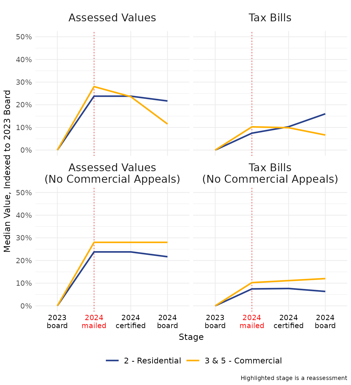
Holding commercial assessments constant makes their effect on residential tax bills clearer: large commercial appeals shift the property tax burden back to residential property owners. In the case of Chicago, the drop in commercial AVs during the second level of review (at the Board of Review) contributed to a roughly 9% rise in the median residential tax bill.

Whether or not this is correct is mostly a matter of interpretation. If the Assessor’s commercial values are accurate, then the subsequent appeals unjustly shifted tax burden back to residential properties. If the Board of Review’s post-appeal values are accurate, then their appeals rightly reversed the unjust increase in commercial tax bills resulting from the 2024 reassessment.

PTAXSIM doesn’t offer a definitive answer or make any normative claims, but it’s an incredibly useful tool for weighing the effects and trade-offs associated with appeals.